Adding background music to Conway’s Game of Life

Conway’s Game of Life never ceases to amaze with the complex patterns that arise from its deceivingly simple rule set. An infinite, two-dimensional orthogonal grid of square cells, each of which is in one of two possible states, alive or dead. A cruel place where lonely cells die and happy cells reproduce. The rules are as follows:

Every cell interacts with its eight neighbours, which are the cells that are horizontally, vertically, or diagonally adjacent. At each step in time, the following transitions occur:

1. Any live cell with fewer than two live neighbours dies, as if by underpopulation.
2. Any live cell with two or three live neighbours lives on to the next generation.
3. Any live cell with more than three live neighbours dies, as if by overpopulation.
4. Any dead cell with exactly three live neighbours becomes a live cell, as if by reproduction.

Wikipedia, Conway’s Game of Life

Implementing the game

Implementing the game’s algorithm in Python is actually pretty easy:

import numpy as np

def update(frameNum, img, grid, N): 
    newGrid = grid.copy() 
    for i in range(N): 
        for j in range(N): 
            # for each pixel calculate the 8-neighbor sum incorporating the needed wrap-around of x and y
            total = int((grid[i, (j-1)%N] + grid[i, (j+1)%N] + 
                         grid[(i-1)%N, j] + grid[(i+1)%N, j] + 
                         grid[(i-1)%N, (j-1)%N] + grid[(i-1)%N, (j+1)%N] + 
                         grid[(i+1)%N, (j-1)%N] + grid[(i+1)%N, (j+1)%N])/255) 
  
            if grid[i, j]  == 255: 
                if (total < 2) or (total > 3): 
                    newGrid[i, j] = 0 
            else: 
                if total == 3: 
                    newGrid[i, j] = 255 
  
    img.set_data(newGrid) 
    grid[:] = newGrid[:]

def randomGrid(size): 
    return np.random.choice((255, 0), size*size, p=[0.2, 0.8]).reshape(size, size) #return a random grid with more pixels off than on

For obvious reasons, instead of a truly infinite grid, we use a finite, square grid that wraps around to form a torus-like surface.
To test the two functions we can generate and plot a random grid and then plot it again after running update():

import matplotlib.pyplot as plt 

grid = np.array([]) 
grid = randomGrid(100) 
fig, ax = plt.subplots(figsize=(9,9))
img = ax.imshow(grid, interpolation='nearest', cmap='Greys_r')

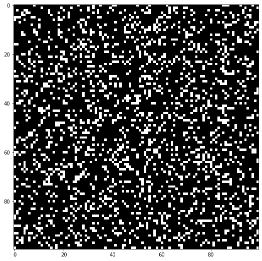
update(2, img, grid, 100)
fig, ax = plt.subplots(figsize=(9,9))
img = ax.imshow(grid, interpolation='nearest', cmap='Greys_r')

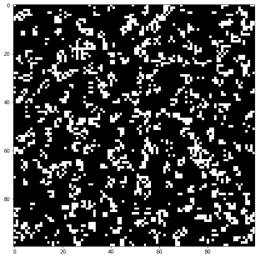
For example we can see how the cell at (0, 0) which is initially dead and has precisely 3 neighbours (at (1, 100), (100, 0) and (100, 100)) becomes alive in the second snapshot.

Adding music to the mix

Many people have used Conway’s Game of Life to produce music, but I had something different in mind.
I realized that, to people that didn’t understand the rules or weren’t as interested in dumb mathematical games as I was, the simple black and white GIFs and videos that we usually use to showcase the game appeared very dull. One solution would be making cells more colorful, but that would either involve messing with the underlying rules of the game, or adding a huge amount of randomness, fundamentally altering the game either way. Another solution, which I finally decided to implement, would be to sync the game to music, updating the grid according to the rhythm of the music.

Attempt #1 — Using rhythm detection

To make the game respond to music I first had to find a way to get meaningful information (from a computer’s perspective) out of the actual sound clips. The first and simplest thing I naturally thought about was tempo (bpm).

import IPython # for interactive previews of audio clips and videos
import moviepy.editor as mpe # for combining audio and video tracks
import essentia.standard as es # for analysis of the audio tracks

For testing I’m using a small clip from the song Feel Good by Syn Cole provided for free by NoCopyrightSounds:

song_filepath = 'audio/feelgood_crop.wav'

audio = es.MonoLoader(filename=song_filepath)()
duration = len(audio)/44100.0 #in seconds
print("Song duration: {:.2f} sec".format(duration))
IPython.display.Audio(song_filepath)

Song duration: 31.00 sec

To extract the bpm value straight from the sound clip I used a super cool open-source library called Essentia, that provides very easy to use Python bindings.
Using the RhythmExtractor2013 algorithm we get predictions for the bpm of the song as well as the precise location of each detected beat:

rythm_extractor = es.RhythmExtractor2013(method="multifeature")
bpm, beats, beats_confidence, _, beats_intervals = rythm_extractor(audio)

print("BPM: {:.2f}\nFirst beat at {:.2f} sec".format(bpm, beats[0]))

BPM: 123.90
First beat at 0.50 sec

We can try to visualize the detected beats by plotting both the waveform of the audio and the estimated beat positions (red lines):

from pylab import plot, show, figure, imshow
import matplotlib.pyplot as plt
plt.rcParams['figure.figsize'] = (15, 6)

plot(audio)
for beat in beats:
    plt.axvline(x=beat*44100, color='red')

plt.title("Audio waveform and estimated beat positions")
plt.show()

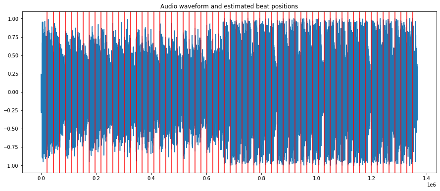
This does not really give us any useful information about the predicted beat locations. To see if the algorithm really predicts the correct locations we can instead mark each of those locations with a distinctive beep sound and listen to the result:

marker = es.AudioOnsetsMarker(onsets=beats, type='beep')
marked_audio = marker(audio)
es.MonoWriter(filename='audio/export.mp3')(marked_audio)

IPython.display.Audio('audio/export.mp3')

And indeed we can hear that the algorithm did a pretty good job at predicting the beat locations and the tempo of the song.

For songs with a constant tempo, like the one I’m using for testing, we can in fact ignore the beat positions and only use the bpm value.
We can now make our first attempt at putting everything together:

# movement(frames) per beat
mpb = 1

import matplotlib.pyplot as plt  
import matplotlib.animation as animation
from math import ceil

fps = int(mpb * bpm / 60)

# Yet again we start with a random grid
grid = np.array([]) 
grid = randomGrid(100) 

fig, ax = plt.subplots(figsize=(15,15))
img = ax.imshow(grid, interpolation='nearest', cmap='Greys_r')
ani = animation.FuncAnimation(fig, update, fargs=(img, grid, 100, ), 
                              frames = ceil(fps * duration), 
                              interval=1, 
                              save_count=50);

ani.save('temp/render.mp4', fps=fps, extra_args=['-vcodec', 'libx264'])
plt.close()

After rendering the animation we pass the clip to moviepy to add the background music:

my_clip = mpe.VideoFileClip('temp/render.mp4')
audio_background = mpe.AudioFileClip(song_filepath)
final_clip = my_clip.set_audio(audio_background)

final_clip.write_videofile("save/output1.mp4", verbose=False)

And we can finally preview the result:

IPython.display.Video('save/output1.mp4', width=625, embed=True)

The result, even if not that stunning, is very much a success! The movement does truly seem to follow the tempo of the song, so mission accomplished right?
Well, not really.
Even though this method works pretty well for songs with a constant tempo, when we try using it for other songs we start seeing its limitations.
One of the best examples for this is a piano composition called Sad Day by Benjamin Tissot (provided for free by bensound.com).

This is how the predicted beats for this song sound like:

IPython.display.Audio('audio/sadday-export.mp3')

At this point it was easy to tell that bpm was not really the best metric for achieving my goal. Even though the tempo does appear to be accurate for some parts of the clip, the overall feel of the song is certainly not being portrayed. A sad song like this should not result in a fast animation.
From this point on, the goal was to find a way to get better results across multiple types of music. To make sure I was making progress I decided to use the piano track as a test song for all following attempts.

Generalizing the video creation algorithm

Let’s load the new clip and start working on a better solution.

song_filepath = 'audio/sadday_crop.wav'

audio = es.MonoLoader(filename=song_filepath)()
duration = len(audio)/44100.0 #in seconds
print("Song duration: {:.2f} sec".format(duration))
IPython.display.Audio(song_filepath)

Song duration: 29.22 sec

The first thing that I had to do was finding a consistent way of going from a song and a list of timestamps (e.g. of beats) to a video. To achieve this I created this simple function that first generates all frames needed and saves them to disk and then takes those frames, converts them to clips and combines them all to create a video. This allows us to only switch frames when we reach a new timestamp and totally avoid average values (like bpm).

def animate(timestamps, output_filepath, audiofile=song_filepath):
    grid = np.array([]) 
    grid = randomGrid(100) 

    fig, ax = plt.subplots(figsize=(15,15))
    img = ax.imshow(grid, interpolation='nearest', cmap='Greys_r')

    # generate and save to disk all consecutive frames needed to make the animation
    for i in range(0, len(timestamps) - 1):
        update(i, img, grid, 100)
        plt.savefig("temp/img{}.jpg".format(i))
    
    plt.close()

    # transform those frames to clips with the needed duration
    clips = []
    for i in range(len(timestamps) - 1):
        dur = timestamps[i+1] - timestamps[i] # the duration of the clip is as much as the time between this and the next timestamp
        newclip = mpe.ImageClip("temp/img{}.jpg".format(i)).set_duration(dur)
        clips.append(newclip)
    
    # combine all clips to one
    concat_clip = mpe.concatenate_videoclips(clips, method="compose")
    
    # add the background music and export
    audio_background = mpe.AudioFileClip(audiofile)
    final_clip = concat_clip.set_audio(audio_background)
    final_clip.write_videofile(output_filepath, fps=24)

To test this we can calculate the beat positions of our new sample song and using the output generate a video:

bpm, beats, beats_confidence, _, beats_intervals = rythm_extractor(audio)
animate([0] + beats.tolist() + [duration], "save/output2.mp4")

IPython.display.Video('save/output2.mp4', width=625, embed=True)

The result is as disappointing as I expected (because we are still using beats) but at least we now have a more generalizable way of producing these videos.
Now the only thing that remains is finding an algorithm that returns more meaningful timestamps for our songs.

Attempt #2 — Using onset detection

Looking through different examples from Essentia’s documentation I stumbled upon a way to detect onset locations for a given track (Onset detection) which at a quick glance seemed like a way better idea than just using beat detection.
Wikipedia defines an onset as "The beginning of a musical note or other sound" which actually further increased my expectations. The only problem is that onset detection is still an active research area and the algorithms aren’t quite that good yet.
Either way I decided to give it a try.

The following code, found in Essentia’s documentation gives us a list of timestamps of detected onsets:

import essentia
import essentia.standard as es

audio = es.MonoLoader(filename=song_filepath)()

od1 = es.OnsetDetection(method='hfc')

w = es.Windowing(type = 'hann')
fft = es.FFT()
c2p = es.CartesianToPolar()
pool = essentia.Pool()


for frame in es.FrameGenerator(audio, frameSize = 1024, hopSize = 512):
    mag, phase, = c2p(fft(w(frame)))
    pool.add('features.hfc', od1(mag, phase))

# Compute the actual onsets locations
onsets = es.Onsets()

onsets_hfc = onsets(essentia.array([ pool['features.hfc'] ]), [ 1 ])

And we can once again preview their locations using beeps:

marker = es.AudioOnsetsMarker(onsets=onsets_hfc, type='beep')
marked_audio = marker(audio)
es.MonoWriter(filename='save/onsets.mp3')(marked_audio)

IPython.display.Audio('save/onsets.mp3')

Now this is more like it! The beeps do actually seem to indicate the beginning of musical notes and also portray the overall feel of the song much better. The only thing left to do now is to create the video:

animate([0] + onsets_hfc.tolist() + [duration], "save/output3.mp4")

IPython.display.Video('save/output3.mp4', width=625, embed=True)

Awesome! Now you can almost see the sadness in the video.